Prologue

In the last post, we introduced the basics of RL—action, reward, state, value, policy, model, etc.—so you should now have a rough picture of the field. In this post, we go deeper and discuss a classic yet still active topic: Multi-Armed Bandits (MAB). There will be more math ahead; hope you can enjoy it.

Problem Formulation

Multi-armed bandits are popular gambling games. There are slot machines, each called a bandit, with an unknown reward distribution that governs how much you get when pulling its arm. Your goal is to maximize the total winnings within a fixed number of pulls. You may try the game to get an intuition at https://su-my.github.io/Test-page.

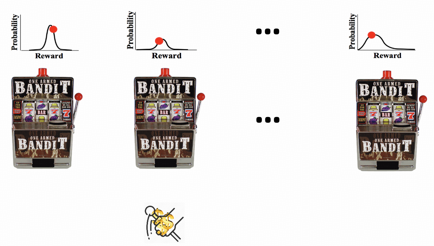
Let’s abstract the gambling game to a formal problem definition:

where the $R_i$ notations are random variabes for rewards.

Furthur discussions:

Regret

Definitions

Regret is the primary metric for evaluating a MAB algorithm. Informally, it is the gap between the reward you would obtain by always pulling the best arm and the reward actually obtained by the algorithm. A smaller regret indicates a better algorithm.

Throughout this section we assume a stochastic environment with arm-wise reward means $\{\mu_k\}_{k=1}^K$, and we write $\mu^* = \max\limits_{1\le k\le K} \mu_k$ for the optimal mean.

The three regret notions above may look verbose, but they separate measurables cleanly and avoid mixing pathwise quantities with expectations¹. Two remarks:

1. $$ \mathbf R^{\mathrm{real}}_\pi(T,\omega) = \sum_{t=1}^T \bigl(r_t(a^*) - r_t(A_t(\omega))\bigr). $$$$ \mathbb E\bigl[\mathbf R^{\mathrm{real}}_\pi(T,\omega)\mid A_1(\omega),\dots,A_T(\omega)\bigr] = \mathbf R_\pi(T,\omega). $$

   In analysis we usually work with pseudo‑regret, and when context is clear we simply say “regret”.

2. Why is $A_t$ random?
   Because both the rewards and the policy may be stochastic. Rewards influence the history observed by the policy, and the policy may randomize given that history; therefore $A_t:\Omega\to\mathcal A$ is a random variable.

Lower Bounds

For convenience, we only talk about the realized regret under a fixed trajectory $\omega$ and a fixed policy $\pi$ and simplify the $\mathbf {R}_\pi(T,\omega)$ as $\mathbf R(T)$.

As mentioned before, we should make the regret grow slower. So what is the lower bound for regret?

It’s easy to find out any algorithm cannot be worse than linear, since:

Hence, a wise algorithm should be sub-linear, i.e. $o(T)$. Two common lower bounds are:

• Gap-independent: $$\Omega(\sqrt{TK})$$
• Gap-dependent: $$\Omega\left(\sum_{a_i \ne a^*} \left( \frac{\Delta_i}{KL(P_{a_i}, P_{a^*})} \right) \log T\right)$$

where $K$ is the number of arms; $\Delta_i$ is the gap between the mean of $a_*$ and $a_i$; the gap-independent means it’s hard to identify the gap between the arms; gap-dependent is the opposite.

Intuitively, the easier the gap is to indentify, the less attention will be paid to find out the best arm and we will get lower regret. That’s why the gap-dependent lower bound is $\Omega(\log T)$ which is less than $\Omega(\sqrt{T})$

Proofs will be provided once I figured them out.

Explore-Exploit Dilemma

The difficulty of MAB comes from the explore-exploit dilemma, which is intuitive once you get to know what MAB problems are chasing for.

• Explore: we must pay some steps to explore the best policy for choosing among arms to avoid commiting to the wrong arms causing linear regrets later. But the exploration phase is always along with regret accumulation itself because of the wrong attempts we must meet.
• Exploit: Stick to current policy. As talked before, this may leads to high regret if the exploration is not sufficient.

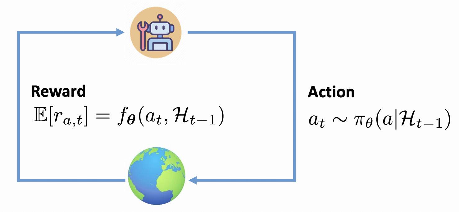
MAB From the Perspective of RL

As the broad picture you may have for MAB now, it’s just a RL-like problem with simplified environments. You may treat the reward in MAB as a combination of observation and reward in RL.

Tail Bounds²

To get into the real discussion of MAB, we first state a few mathematical propositions that describe how far samples of a random variable can deviate from its expectation. This is necessary for further analysis of MAB algorithms since we are estimating the means $\mu_k$; if we can estimate these means accurately and quickly, we can obtain low regret.

If you are not interested in the math details, you can jump to Hoeffding’s Inequality and skip this section omitting all proofs.

Markov’s Inequality

Chebyshev’s Inequality

Chernoff Bound

The Chernoff bound is a technique to estimate tail bounds quantitatively, i.e., $\Pr(X\ge a)$ or $\Pr(X\le a)$. We can summarize it in three steps:

As an illustration, consider Bernoulli trials and apply the Chernoff bound.

Suppose we have $n$ i.i.d. Bernoulli trials $X_i$ with success probability $p$. Let $X=\sum_i X_i$; then $\mu = \mathbb E[X]=np$. Suppose $\lambda > 1$.

where $D_{\text{KL}}(q\parallel p)= q\log\!\frac{q}{p} + (1-q)\log\!\frac{1-q}{1-p}$ is the Kullback–Leibler divergence between Bernoulli parameters.

Hoeffding’s Inequality

The protagonist finally comes! The Hoeffding’s inequality are bounding a set of independent bounded random variables. You may find it especially useful in MAB problems since the arms are basically a set of independent random variables.

Hoeffding’s Inequality is actually a special case of Chernoff Bound. Let’s give the proposition first:

It’s easy to find out the Hoeffding’s inequality is a special case of Chernoff Bound.

We used Hoeffding’s Lemma to bound the MGF of $X_i-\mu_i$:

Let’s also give a special case of Hoeffding’s Inequality here when all random variables are i.i.d. and sub-gaussian.

Explore-Then-Commit

Explore-Then-Commit (ETC) is an intuitive algorithm for MAB problems. It pulls each arm a fixed number of times, then commits to the arm with the highest estimated mean.

Consider the special case where all arms are $1$-sub-Gaussian; this helps build intuition for the regret. For brevity, we denote the expected pseudo-regret of ETC at horizon $n$ by $R_{\mathrm{ETC}}(n)$.

W.l.o.g., assume $\forall i < j, \mu_i \ge \mu_j$, and define $\Delta_i = \mu_1 - \mu_i$.

The first inequality is strict when multiple arms tie, because the tie-breaking rule is random. The last inequality follows since $X-Y$ is $\sqrt{2}$-sub-Gaussian when $X$ and $Y$ are $1$-sub-Gaussian, and then we can apply the Hoeffding’s Inequality.

which implies

Note that $m \ge 1$, and $R_{\operatorname{ETC}(m)} (n)$ cannot exceed $n\Delta$ as discussed above. Informally, this bound says that, for fixed gap $\Delta$, the regret of ETC grows only logarithmically with the horizon $n$, but with a relatively large constant and the need to know (or tune around) $\Delta$ to choose $m$.

We can plot how $R_{\operatorname{ETC}} (n)$ changes with $\Delta$ using a short Python snippet:

import numpy as np
import matplotlib.pyplot as plt

n = 1000
eps = 1e-6
deltas = np.linspace(eps, 100.0, 1000)

term_linear = n * deltas
term_log = deltas + (4 / deltas) * (1 + np.maximum(0, np.log(n * deltas**2 / 4)))
bound = np.minimum(term_linear, term_log)

plt.figure(figsize=(6, 4))
plt.plot(deltas, bound, label=r"$R_{\mathrm{ETC}}(n)$ upper bound")
plt.xlabel(r"$\Delta$")
plt.ylabel(r"regret bound")
plt.title(f"ETC regret bound vs Δ (n={n})")
plt.grid(True, ls="--", alpha=0.5)
plt.legend()
plt.tight_layout()
plt.show()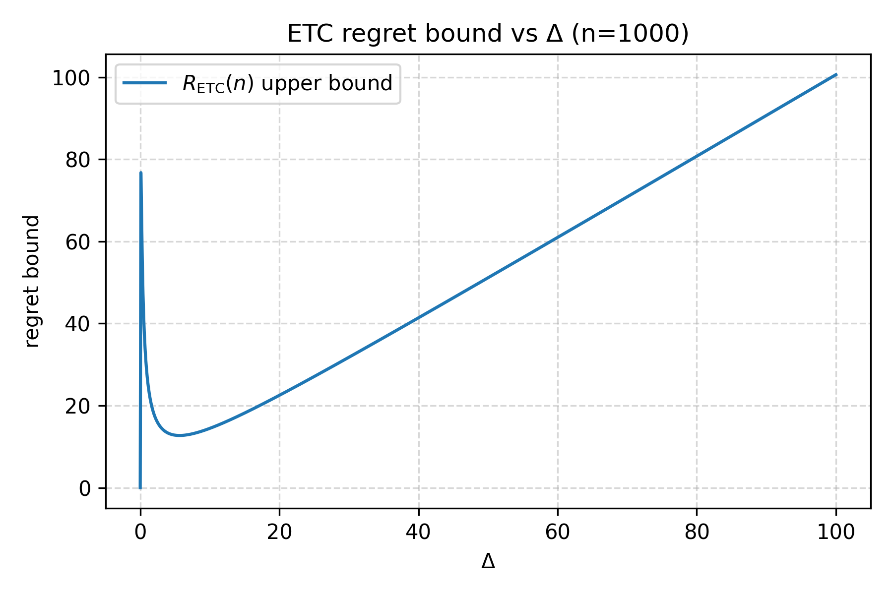

The regret bound diverges as $\Delta \to \infty$. If we restrict to $\Delta \le 1$ (arms are $1$-sub-Gaussian), the bound is maximized near $\Delta \approx \frac{2\sqrt{e}}{\sqrt{n}}$, where $R_{\operatorname{ETC}} (n) \approx \frac{4\sqrt{n}}{\sqrt{e}}$ (from differentiating the RHS with respect to $m$). For fixed $\Delta$, the gap-dependent upper bound scales as $O((\log n)/\Delta)$, but unlike UCB it needs a good estimate of $\Delta$ (to choose $m$) and carries larger constants.

Varaints of ETC

ETC is intuitive but too simple, which leads to the folloing disadvatages:

1. It requires the prior of $\Delta$ to find the best $m$ for exploration, which are usually unknown in real scenerios.
2. It is too rigid. It may continually commit to the wrong arms in the exploration phase.
3. Theorectically, it is usually two times of the gap-dependent lower bound.

Hence, there are two common variants of ETC to address the above disadvantages:

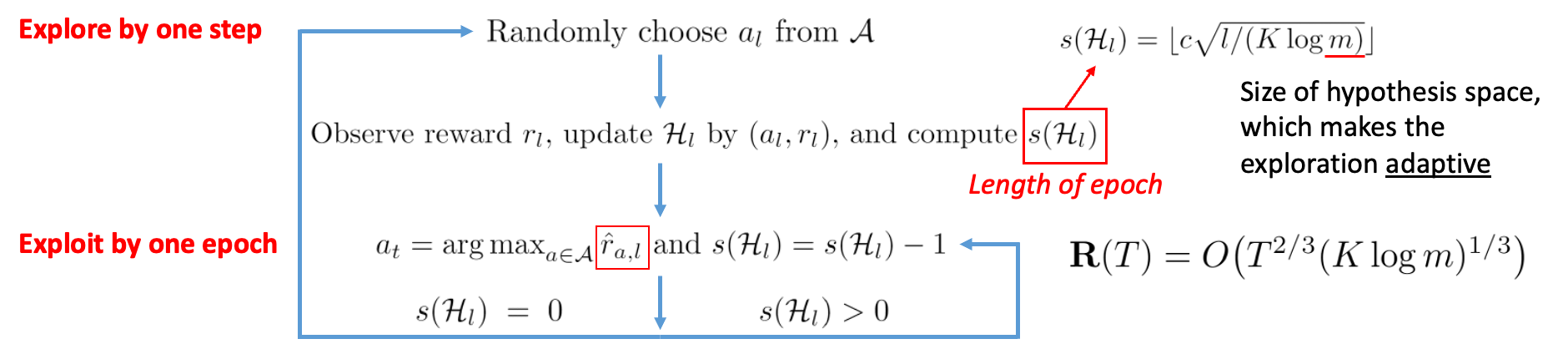
Epoch Greedy ETC

Rather than committing to the arm with the highest estimated mean, Epoch Greedy ETC commits to the arm with the highest estimated mean in each epoch.

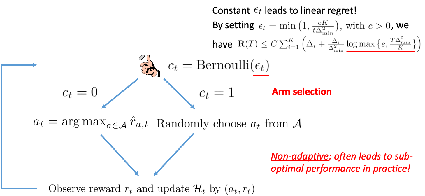
$\varepsilon$-Greedy ETC

Toss a coin with probability $\varepsilon$ to commit to the arm with the highest estimated mean, otherwise commit to a random arm.

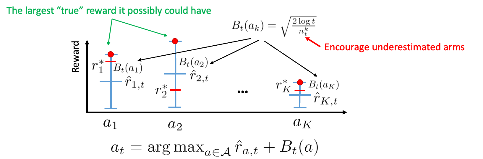
Upper Confidence Bound (UCB)

UCB is a classical algorithm for MAB problems. It follows the optimism‑in‑the‑face‑of‑uncertainty principle: arms with larger statistical uncertainty receive a positive bonus, so rarely sampled arms are explored more.

Throughout this subsection we write $R_{\mathrm{UCB}}(n)$ for the expected pseudo-regret of the UCB algorithm at horizon $n$.

The bonus $B_t(a)$ shrinks as $N_t(a)$ grows and increases slowly with $t$, encouraging exploration of under‑sampled arms.

The form of $B_t(a)$ comes directly from Hoeffding’s Inequality.

Next we sketch the regret of UCB. Assume all arms are $\tfrac{1}{2}$‑sub-Gaussian, and $\beta = 4$, hence $\alpha = 2$. Order the arms so that $\mu_1 \ge \mu_2 \ge \cdots \ge \mu_k$ and define the gaps $\Delta_i = \mu_1 - \mu_i$ for $i\ge2$.

so the contribution from the “bad” events $\neg G_t$ is a constant independent of $n$.

Putting this together with the ETC analysis above, both $R_{\mathrm{ETC}}(n)$ and $R_{\mathrm{UCB}}(n)$ achieve a gap‑dependent logarithmic rate $O((\log n)/\Delta)$, but ETC needs a well‑tuned exploration length $m$ (which in turn depends on the unknown gap), whereas UCB attains the same order of regret without any prior knowledge of $\Delta$ by adapting its exploration bonus online.